Lab 21: Spectrum of a Real Sound

Time: ~50 minutes | Prerequisites: Lab 20 | Hardware: Pico 2, INMP441, OLED

This is the one you've been building toward

Fourteen labs of groundwork, and now it all points outward. Microphone in, FFT, bars on the screen. Then whistle at it and slide your pitch around — the peak follows you. That's a sound becoming a number you can see. Now that's a superpower.

What You'll Build

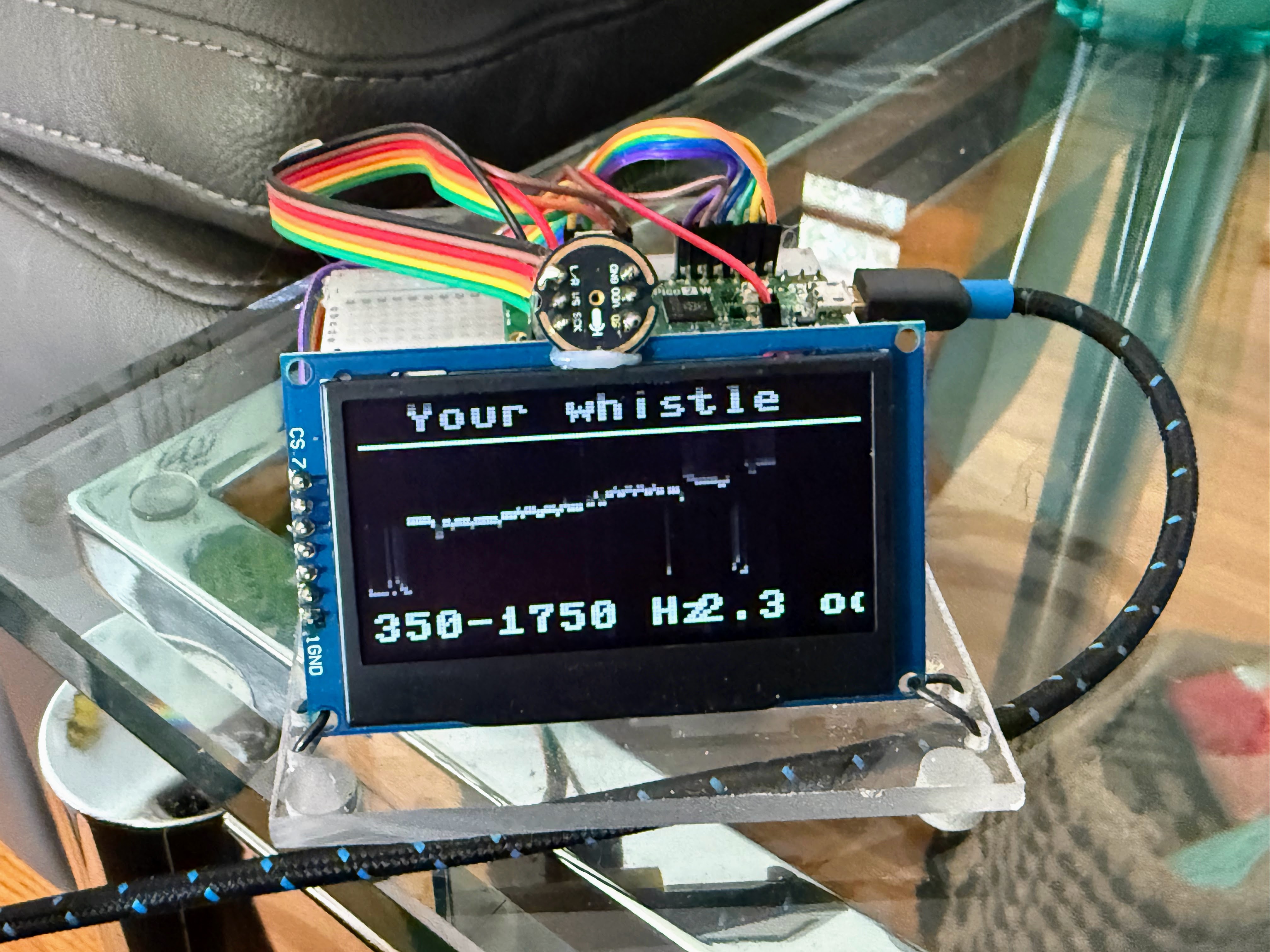
A live spectrum analyzer: real audio in, a 32-bar display out, with a peak-frequency readout that tracks your whistle.

Learning Objectives

• Connect the microphone, FFT and display into one pipeline
• Import your FFT as a library rather than pasting it
• Convert a complex spectrum to magnitudes, cheaply
• Group bins into display bars and scale them sensibly
• Explain why a quiet room's spectrum slopes downward
• Reject low-frequency rumble when hunting for a peak

Concepts Introduced

ID	Concept
400	Magnitude Computation
401	Fast Magnitude Approximation
402	Power Versus Magnitude
403	Bin Averaging For Display
404	Logarithmic Scaling
405	Square Root Scaling
406	Spectrum Bars
407	Frame Capture
408	Live Spectrum Display
409	Whistle Test
410	Half Spectrum Display

Background

Your FFT is now a library

The FFT you built in Lab 20 lives in /lib/fftlab.py. Same algorithm, nothing added:

from fftlab import FFT
fft = FFT(256)
re, im = fft.buffers()
fft.run(re, im)
mags = fft.fast_magnitudes(re, im)

You're using a library whose entire contents you wrote and validated — a far better position than trusting a black box.

Magnitude, without the square root

True magnitude needs sqrt(re² + im²), and square roots aren't cheap. When the answer becomes a bar 40 pixels tall, this approximation is plenty:

|z| ≈ max(|re|,|im|) + 0.4 · min(|re|,|im|)

Within about 4%, noticeably faster. Knowing when precision doesn't matter is an engineering skill.

Why N = 256 here

At N = 512 the pure-Python FFT takes 145 ms — about 7 frames per second, which feels sluggish. N = 256 takes ~71 ms and feels alive.

The cost: bins are 50 Hz wide instead of 25. Resolution traded for speed — a tradeoff you'll meet formally in Lab 24 and finally beat in Module 7.

Rooms rumble

Point this at a silent room and the spectrum slopes steeply downward — bin 2 towering over everything. That's 1/f noise: traffic, ventilation, the building itself. It's real sound, not a bug. But it means the loudest bin is always low-frequency rumble, which would drown out any whistle. So we start hunting above 300 Hz.

Procedure

Step 1 — Run it and whistle

Open 21-real-spectrum.py and run it:

# Lab 21: Spectrum of a Real Sound
#
# THIS IS THE PAYOFF.
#
# Everything since Lab 7 has been building toward this: point the microphone
# at the world, transform what it hears, and draw the frequencies on screen.
#
# Then whistle at it. Slide your pitch up and down and watch the peak move.
# That moment -- when a sound becomes a NUMBER you can see -- is what the
# whole course is about.

import config
import math
import struct
import time
from fftlab import FFT

N = 256                       # smaller than 512 so the display stays lively
RATE = config.SAMPLE_RATE     # 12800 Hz
BIN_HZ = RATE / N             # 50 Hz per bin

# Rooms are full of low-frequency rumble -- traffic, fans, your own
# building. It falls off as 1/f, so bin 1 or 2 almost always "wins" even in
# silence. We ignore everything below this bin when hunting for a peak.
MIN_BIN = 6                   # 300 Hz -- above the rumble, below a whistle
PEAK_RATIO = 3.0              # a real peak must stand this far above average

BARS = 32                     # bars across the 128-pixel display
BAR_W = config.WIDTH // BARS
TOP = 14                      # leave room for the title
BAR_H = config.HEIGHT - TOP - 10

fft = FFT(N)
oled = config.init_display()
mic = config.init_microphone()
raw = bytearray(N * 4)
re, im = fft.buffers()

print("Settling the microphone...")
for _ in range(5):
    mic.readinto(raw)
    time.sleep_ms(50)

print()
print("=== Live spectrum ===")
print("bin width : %.0f Hz" % BIN_HZ)
print("range     : 0 to %.0f Hz" % (RATE / 2))
print()
print("WHISTLE AT IT. Slide your pitch up and down and watch the peak move.")
print("Ctrl-C to stop.")
print()


def capture():
    """Read one frame of audio into the FFT's real buffer."""
    n = mic.readinto(raw)
    words = struct.unpack("<%di" % (n // 4), raw[:n])
    count = min(N, len(words))
    # Remove the DC offset (Lab 7) -- otherwise bin 0 swamps everything.
    total = 0
    for i in range(count):
        total += words[i] >> 8
    dc = total / count
    for i in range(count):
        re[i] = (words[i] >> 8) - dc
        im[i] = 0.0
    for i in range(count, N):
        re[i] = 0.0
        im[i] = 0.0


def find_peak(mags):
    """Loudest bin above the rumble, but only if it really stands out.

    Returns (bin, hz) or (None, 0) when nothing convincing is present.
    """
    top = N // 2
    total = 0.0
    for k in range(MIN_BIN, top):
        total += mags[k]
    average = total / (top - MIN_BIN)

    best_k = MIN_BIN
    best_v = 0.0
    for k in range(MIN_BIN, top):
        if mags[k] > best_v:
            best_v = mags[k]
            best_k = k

    if best_v < PEAK_RATIO * average:
        return None, 0.0        # just noise -- no honest answer to give
    if best_k == MIN_BIN:
        # The winner is sitting right on the edge of the rumble we excluded.
        # That is nearly always the rumble leaning in, not a real tone --
        # you can see it in a pitch track as spurious readings during the
        # gaps when the whistler takes a breath.
        return None, 0.0
    return best_k, best_k * BIN_HZ


def draw(mags, peak_bin, peak_hz):
    oled.fill(config.BLACK)
    if peak_bin is None:
        oled.text("  listening", 0, 0, config.WHITE)
    else:
        oled.text("%5d Hz" % peak_hz, 0, 0, config.WHITE)
    oled.hline(0, 11, config.WIDTH, config.WHITE)

    # Group the bins into display bars. We only plot the lower part of the
    # spectrum -- most interesting sound lives below a few kHz.
    usable = N // 2
    per_bar = usable // BARS
    biggest = 1.0
    heights = []
    for b in range(BARS):
        s = 0.0
        for k in range(b * per_bar, (b + 1) * per_bar):
            if mags[k] > s:
                s = mags[k]
        heights.append(s)
        if s > biggest:
            biggest = s

    for b, h in enumerate(heights):
        # Square-root scaling: makes quiet detail visible without a log.
        norm = math.sqrt(h / biggest)
        px = int(norm * BAR_H)
        if px > 0:
            oled.fill_rect(b * BAR_W, TOP + BAR_H - px, BAR_W - 1, px,
                           config.WHITE)

    # Mark the peak bar, when there is one worth marking.
    if peak_bin is not None:
        pb = min(BARS - 1, peak_bin // per_bar)
        oled.fill_rect(pb * BAR_W, config.HEIGHT - 8, BAR_W - 1, 3, config.WHITE)
    oled.show()


try:
    while True:
        capture()
        fft.run(re, im)
        mags = fft.fast_magnitudes(re, im)

        peak_bin, peak_hz = find_peak(mags)

        draw(mags, peak_bin, peak_hz)
        if peak_bin is None:
            print("listening... (no clear tone)")
        else:
            print("peak: bin %3d = %5.0f Hz" % (peak_bin, peak_hz))

except KeyboardInterrupt:
    mic.deinit()
    oled.fill(config.BLACK)
    oled.text("Stopped.", 32, 28, config.WHITE)
    oled.show()
    print("Stopped.")

peak: bin   6 =   300 Hz
peak: bin  31 =  1550 Hz
peak: bin  34 =  1700 Hz

Now whistle. Start low and slide upward. The bar moves right and the number climbs. Slide back down and it follows.

That's the FFT working on the real world, in real time, on a $5 chip.

Step 2 — Try different sounds

Sound	What to look for
Whistle	one sharp peak that tracks your pitch
Humming	a peak plus harmonics — evenly spaced taller bars
"Sssss"	broad energy spread across high bins, no peak
Clapping	everything lights up briefly (Lab 15's impulse!)
Silence	rumble at the left, "listening" on screen

Humming is the interesting one. Your voice isn't a pure tone — it's a fundamental plus overtones, exactly the additive recipe from Lab 12, now visible.

Step 3 — Understand the peak-finder

if best_v < PEAK_RATIO * average:
    return None, 0.0        # just noise -- no honest answer to give

Two safeguards. MIN_BIN skips the rumble. PEAK_RATIO demands the peak stand three times above average before we believe it — otherwise the display says "listening" rather than inventing a frequency.

Reporting nothing beats reporting nonsense

A meter that always shows a number looks confident and is often lying. One that admits "no clear tone" is more useful — and it's the same instinct as Lab 9's aliasing lesson. Know when your instrument has nothing to say.

Step 4 — Square-root scaling

norm = math.sqrt(h / biggest)

Raw magnitudes are dominated by the loudest bin and everything else vanishes. Square root compresses the range so quiet detail stays visible, without the expense of a log. Try removing it — the display goes almost blank between peaks.

Step 5 — Predict, then measure

Prediction: whistle a steady note. How many different bins does the reading jump between? Why doesn't it hold perfectly still?

You've just discovered frequency resolution, which is Lab 23's whole problem.

Expected Output

Thirty-two bars responding to sound, a peak-frequency readout, and a marker under the peak bar. Silence shows "listening".

Troubleshooting

Symptom	Likely cause	Fix
Always shows "listening"	PEAK_RATIO too high, or too quiet	Lower it to 2.0, or whistle louder
Peak stuck at the lowest bin	MIN_BIN too low	Raise toward 8
Bars all maxed out	Normalising to the wrong value	biggest should be the max across bars
Very sluggish	N too large	256 is the sweet spot in pure Python
Bin 0 enormous	DC not removed	Subtract the mean (Lab 7)
ImportError: fftlab	Library not on the board	It belongs in /lib

Challenges

1. Peak hold. Keep the highest peak seen in the last two seconds and mark it, like Lab 8's VU meter.
2. Waterfall. Scroll the display downward each frame, drawing brightness by magnitude. You'll have built a spectrogram.
3. Count the harmonics. Hum a steady note and count evenly-spaced peaks. Does the spacing match your fundamental?

Check Your Understanding

1. Why is a quiet room's spectrum loudest at low frequencies?
2. Why does the peak-finder ignore bins below 300 Hz?
3. What does the fast magnitude approximation trade away, and why is that acceptable here?
4. Why does square-root scaling make the display more readable?
5. Humming shows several evenly-spaced peaks. What are they?

You made a sound into a picture

Fourteen labs ago you couldn't tell a whistle from a rumble. Now your Pico draws the difference, live. Next lab: why your whistle sometimes smears across several bars instead of making one clean spike.

---

Next: Lab 22: Windowing and Spectral Leakage | Previous: Lab 20